Anotación de parcelas

Los siguientes ejemplos muestran cómo es posible anotar gráficos en Matplotlib. Esto incluye resaltar puntos de interés específicos y usar varias herramientas visuales para llamar la atención sobre este punto. Para obtener una descripción más completa y detallada de las herramientas de anotación y texto en Matplotlib, consulte el tutorial sobre anotación .

import matplotlib.pyplot as plt
from matplotlib.patches import Ellipse
import numpy as np
from matplotlib.text import OffsetFrom

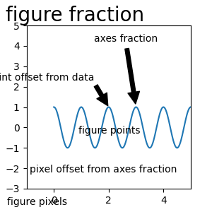
Especificación de puntos de texto y puntos de anotación

Debe especificar un punto de anotación para anotar este punto. Además, puede especificar un punto de texto para la ubicación del texto de esta anotación. Opcionalmente, puede especificar el sistema de coordenadas de xy y xytext con una de las siguientes cadenas para xycoords y textcoords (el valor predeterminado es 'data'):xy=(x, y)xytext=(x, y)

'figure points'   : points from the lower left corner of the figure
'figure pixels'   : pixels from the lower left corner of the figure
'figure fraction' : (0, 0) is lower left of figure and (1, 1) is upper right
'axes points'     : points from lower left corner of axes
'axes pixels'     : pixels from lower left corner of axes
'axes fraction'   : (0, 0) is lower left of axes and (1, 1) is upper right
'offset points'   : Specify an offset (in points) from the xy value
'offset pixels'   : Specify an offset (in pixels) from the xy value
'data'            : use the axes data coordinate system

Nota: para sistemas de coordenadas físicas (puntos o píxeles) el origen es (abajo, a la izquierda) de la figura o ejes.

Opcionalmente, puede especificar propiedades de flecha que dibujen una flecha desde el texto hasta el punto anotado proporcionando un diccionario de propiedades de flecha

Las claves válidas son:

width : the width of the arrow in points
frac  : the fraction of the arrow length occupied by the head
headwidth : the width of the base of the arrow head in points
shrink : move the tip and base some percent away from the
         annotated point and text
any key for matplotlib.patches.polygon  (e.g., facecolor)

# Create our figure and data we'll use for plotting
fig, ax = plt.subplots(figsize=(3, 3))

t = np.arange(0.0, 5.0, 0.01)
s = np.cos(2*np.pi*t)

# Plot a line and add some simple annotations
line, = ax.plot(t, s)
ax.annotate('figure pixels',
            xy=(10, 10), xycoords='figure pixels')
ax.annotate('figure points',
            xy=(80, 80), xycoords='figure points')
ax.annotate('figure fraction',
            xy=(.025, .975), xycoords='figure fraction',
            horizontalalignment='left', verticalalignment='top',
            fontsize=20)

# The following examples show off how these arrows are drawn.

ax.annotate('point offset from data',
            xy=(2, 1), xycoords='data',
            xytext=(-15, 25), textcoords='offset points',
            arrowprops=dict(facecolor='black', shrink=0.05),
            horizontalalignment='right', verticalalignment='bottom')

ax.annotate('axes fraction',
            xy=(3, 1), xycoords='data',
            xytext=(0.8, 0.95), textcoords='axes fraction',
            arrowprops=dict(facecolor='black', shrink=0.05),
            horizontalalignment='right', verticalalignment='top')

# You may also use negative points or pixels to specify from (right, top).
# E.g., (-10, 10) is 10 points to the left of the right side of the axes and 10
# points above the bottom

ax.annotate('pixel offset from axes fraction',
            xy=(1, 0), xycoords='axes fraction',
            xytext=(-20, 20), textcoords='offset pixels',
            horizontalalignment='right',
            verticalalignment='bottom')

ax.set(xlim=(-1, 5), ylim=(-3, 5))

[(-1.0, 5.0), (-3.0, 5.0)]

Uso de múltiples sistemas de coordenadas y tipos de ejes

Puede especificar el punto xy y el texto xy en diferentes posiciones y sistemas de coordenadas y, opcionalmente, activar una línea de conexión y marcar el punto con un marcador. Las anotaciones también funcionan en los ejes polares.

En el ejemplo a continuación, el punto xy está en coordenadas nativas ( el valor predeterminado de xycoords es 'data'). Para ejes polares, esto está en el espacio (theta, radio). El texto del ejemplo está colocado en el sistema de coordenadas de figuras fraccionarias. Se respetan los argumentos de palabras clave de texto como la alineación horizontal y vertical.

fig, ax = plt.subplots(subplot_kw=dict(projection='polar'), figsize=(3, 3))
r = np.arange(0, 1, 0.001)
theta = 2*2*np.pi*r
line, = ax.plot(theta, r)

ind = 800
thisr, thistheta = r[ind], theta[ind]
ax.plot([thistheta], [thisr], 'o')
ax.annotate('a polar annotation',
            xy=(thistheta, thisr),  # theta, radius
            xytext=(0.05, 0.05),    # fraction, fraction
            textcoords='figure fraction',
            arrowprops=dict(facecolor='black', shrink=0.05),
            horizontalalignment='left',
            verticalalignment='bottom')

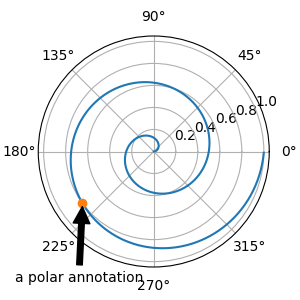
Text(0.05, 0.05, 'a polar annotation')

También puede usar notación polar en ejes cartesianos. Aquí, el sistema de coordenadas nativo ('datos') es cartesiano, por lo que debe especificar xycoords y textcoords como 'polar' si desea usar (theta, radio).

el = Ellipse((0, 0), 10, 20, facecolor='r', alpha=0.5)

fig, ax = plt.subplots(subplot_kw=dict(aspect='equal'))
ax.add_artist(el)
el.set_clip_box(ax.bbox)
ax.annotate('the top',
            xy=(np.pi/2., 10.),      # theta, radius
            xytext=(np.pi/3, 20.),   # theta, radius
            xycoords='polar',
            textcoords='polar',
            arrowprops=dict(facecolor='black', shrink=0.05),
            horizontalalignment='left',
            verticalalignment='bottom',
            clip_on=True)  # clip to the axes bounding box

ax.set(xlim=[-20, 20], ylim=[-20, 20])

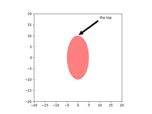
[(-20.0, 20.0), (-20.0, 20.0)]

Personalización de estilos de flechas y burbujas

La flecha entre el texto xy y el punto de anotación, así como la burbuja que cubre el texto de la anotación, son altamente personalizables. A continuación se muestran algunas opciones de parámetros, así como su salida resultante.

fig, ax = plt.subplots(figsize=(8, 5))

t = np.arange(0.0, 5.0, 0.01)
s = np.cos(2*np.pi*t)
line, = ax.plot(t, s, lw=3)

ax.annotate(
    'straight',
    xy=(0, 1), xycoords='data',
    xytext=(-50, 30), textcoords='offset points',
    arrowprops=dict(arrowstyle="->"))
ax.annotate(
    'arc3,\nrad 0.2',
    xy=(0.5, -1), xycoords='data',
    xytext=(-80, -60), textcoords='offset points',
    arrowprops=dict(arrowstyle="->",
                    connectionstyle="arc3,rad=.2"))
ax.annotate(
    'arc,\nangle 50',
    xy=(1., 1), xycoords='data',
    xytext=(-90, 50), textcoords='offset points',
    arrowprops=dict(arrowstyle="->",
                    connectionstyle="arc,angleA=0,armA=50,rad=10"))
ax.annotate(
    'arc,\narms',
    xy=(1.5, -1), xycoords='data',
    xytext=(-80, -60), textcoords='offset points',
    arrowprops=dict(
        arrowstyle="->",
        connectionstyle="arc,angleA=0,armA=40,angleB=-90,armB=30,rad=7"))
ax.annotate(
    'angle,\nangle 90',
    xy=(2., 1), xycoords='data',
    xytext=(-70, 30), textcoords='offset points',
    arrowprops=dict(arrowstyle="->",
                    connectionstyle="angle,angleA=0,angleB=90,rad=10"))
ax.annotate(
    'angle3,\nangle -90',
    xy=(2.5, -1), xycoords='data',
    xytext=(-80, -60), textcoords='offset points',
    arrowprops=dict(arrowstyle="->",
                    connectionstyle="angle3,angleA=0,angleB=-90"))
ax.annotate(
    'angle,\nround',
    xy=(3., 1), xycoords='data',
    xytext=(-60, 30), textcoords='offset points',
    bbox=dict(boxstyle="round", fc="0.8"),
    arrowprops=dict(arrowstyle="->",
                    connectionstyle="angle,angleA=0,angleB=90,rad=10"))
ax.annotate(
    'angle,\nround4',
    xy=(3.5, -1), xycoords='data',
    xytext=(-70, -80), textcoords='offset points',
    size=20,
    bbox=dict(boxstyle="round4,pad=.5", fc="0.8"),
    arrowprops=dict(arrowstyle="->",
                    connectionstyle="angle,angleA=0,angleB=-90,rad=10"))
ax.annotate(
    'angle,\nshrink',
    xy=(4., 1), xycoords='data',
    xytext=(-60, 30), textcoords='offset points',
    bbox=dict(boxstyle="round", fc="0.8"),
    arrowprops=dict(arrowstyle="->",
                    shrinkA=0, shrinkB=10,
                    connectionstyle="angle,angleA=0,angleB=90,rad=10"))
# You can pass an empty string to get only annotation arrows rendered
ax.annotate('', xy=(4., 1.), xycoords='data',
            xytext=(4.5, -1), textcoords='data',
            arrowprops=dict(arrowstyle="<->",
                            connectionstyle="bar",
                            ec="k",
                            shrinkA=5, shrinkB=5))

ax.set(xlim=(-1, 5), ylim=(-4, 3))

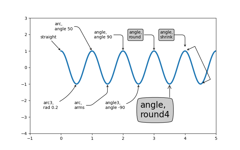
[(-1.0, 5.0), (-4.0, 3.0)]

Crearemos otra figura para que no se abarrote demasiado

fig, ax = plt.subplots()

el = Ellipse((2, -1), 0.5, 0.5)
ax.add_patch(el)

ax.annotate('$->$',
            xy=(2., -1), xycoords='data',
            xytext=(-150, -140), textcoords='offset points',
            bbox=dict(boxstyle="round", fc="0.8"),
            arrowprops=dict(arrowstyle="->",
                            patchB=el,
                            connectionstyle="angle,angleA=90,angleB=0,rad=10"))
ax.annotate('arrow\nfancy',
            xy=(2., -1), xycoords='data',
            xytext=(-100, 60), textcoords='offset points',
            size=20,
            arrowprops=dict(arrowstyle="fancy",
                            fc="0.6", ec="none",
                            patchB=el,
                            connectionstyle="angle3,angleA=0,angleB=-90"))
ax.annotate('arrow\nsimple',
            xy=(2., -1), xycoords='data',
            xytext=(100, 60), textcoords='offset points',
            size=20,
            arrowprops=dict(arrowstyle="simple",
                            fc="0.6", ec="none",
                            patchB=el,
                            connectionstyle="arc3,rad=0.3"))
ax.annotate('wedge',
            xy=(2., -1), xycoords='data',
            xytext=(-100, -100), textcoords='offset points',
            size=20,
            arrowprops=dict(arrowstyle="wedge,tail_width=0.7",
                            fc="0.6", ec="none",
                            patchB=el,
                            connectionstyle="arc3,rad=-0.3"))
ax.annotate('bubble,\ncontours',
            xy=(2., -1), xycoords='data',
            xytext=(0, -70), textcoords='offset points',
            size=20,
            bbox=dict(boxstyle="round",
                      fc=(1.0, 0.7, 0.7),
                      ec=(1., .5, .5)),
            arrowprops=dict(arrowstyle="wedge,tail_width=1.",
                            fc=(1.0, 0.7, 0.7), ec=(1., .5, .5),
                            patchA=None,
                            patchB=el,
                            relpos=(0.2, 0.8),
                            connectionstyle="arc3,rad=-0.1"))
ax.annotate('bubble',
            xy=(2., -1), xycoords='data',
            xytext=(55, 0), textcoords='offset points',
            size=20, va="center",
            bbox=dict(boxstyle="round", fc=(1.0, 0.7, 0.7), ec="none"),
            arrowprops=dict(arrowstyle="wedge,tail_width=1.",
                            fc=(1.0, 0.7, 0.7), ec="none",
                            patchA=None,
                            patchB=el,
                            relpos=(0.2, 0.5)))

ax.set(xlim=(-1, 5), ylim=(-5, 3))

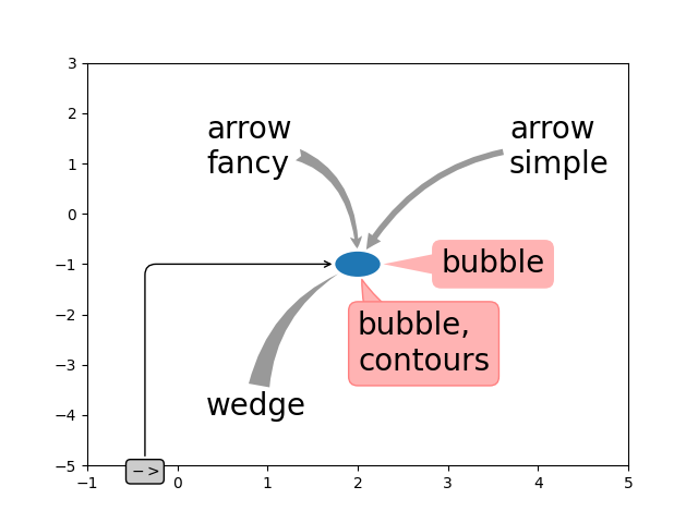
[(-1.0, 5.0), (-5.0, 3.0)]

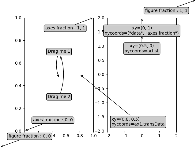
Más ejemplos de sistemas de coordenadas

A continuación, mostraremos algunos ejemplos más de sistemas de coordenadas y cómo se puede especificar la ubicación de las anotaciones.

fig, (ax1, ax2) = plt.subplots(1, 2)

bbox_args = dict(boxstyle="round", fc="0.8")
arrow_args = dict(arrowstyle="->")

# Here we'll demonstrate the extents of the coordinate system and how
# we place annotating text.

ax1.annotate('figure fraction : 0, 0', xy=(0, 0), xycoords='figure fraction',
             xytext=(20, 20), textcoords='offset points',
             ha="left", va="bottom",
             bbox=bbox_args,
             arrowprops=arrow_args)

ax1.annotate('figure fraction : 1, 1', xy=(1, 1), xycoords='figure fraction',
             xytext=(-20, -20), textcoords='offset points',
             ha="right", va="top",
             bbox=bbox_args,
             arrowprops=arrow_args)

ax1.annotate('axes fraction : 0, 0', xy=(0, 0), xycoords='axes fraction',
             xytext=(20, 20), textcoords='offset points',
             ha="left", va="bottom",
             bbox=bbox_args,
             arrowprops=arrow_args)

ax1.annotate('axes fraction : 1, 1', xy=(1, 1), xycoords='axes fraction',
             xytext=(-20, -20), textcoords='offset points',
             ha="right", va="top",
             bbox=bbox_args,
             arrowprops=arrow_args)

# It is also possible to generate draggable annotations

an1 = ax1.annotate('Drag me 1', xy=(.5, .7), xycoords='data',
                   ha="center", va="center",
                   bbox=bbox_args)

an2 = ax1.annotate('Drag me 2', xy=(.5, .5), xycoords=an1,
                   xytext=(.5, .3), textcoords='axes fraction',
                   ha="center", va="center",
                   bbox=bbox_args,
                   arrowprops=dict(patchB=an1.get_bbox_patch(),
                                   connectionstyle="arc3,rad=0.2",
                                   **arrow_args))
an1.draggable()
an2.draggable()

an3 = ax1.annotate('', xy=(.5, .5), xycoords=an2,
                   xytext=(.5, .5), textcoords=an1,
                   ha="center", va="center",
                   bbox=bbox_args,
                   arrowprops=dict(patchA=an1.get_bbox_patch(),
                                   patchB=an2.get_bbox_patch(),
                                   connectionstyle="arc3,rad=0.2",
                                   **arrow_args))

# Finally we'll show off some more complex annotation and placement

text = ax2.annotate('xy=(0, 1)\nxycoords=("data", "axes fraction")',
                    xy=(0, 1), xycoords=("data", 'axes fraction'),
                    xytext=(0, -20), textcoords='offset points',
                    ha="center", va="top",
                    bbox=bbox_args,
                    arrowprops=arrow_args)

ax2.annotate('xy=(0.5, 0)\nxycoords=artist',
             xy=(0.5, 0.), xycoords=text,
             xytext=(0, -20), textcoords='offset points',
             ha="center", va="top",
             bbox=bbox_args,
             arrowprops=arrow_args)

ax2.annotate('xy=(0.8, 0.5)\nxycoords=ax1.transData',
             xy=(0.8, 0.5), xycoords=ax1.transData,
             xytext=(10, 10),
             textcoords=OffsetFrom(ax2.bbox, (0, 0), "points"),
             ha="left", va="bottom",
             bbox=bbox_args,
             arrowprops=arrow_args)

ax2.set(xlim=[-2, 2], ylim=[-2, 2])
plt.show()