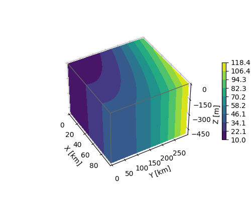
Gráfico de superficie de caja 3D

Dados los datos de un volumen cuadriculado X, Y, Z, este ejemplo traza los valores de los datos en las superficies del volumen.

La estrategia es seleccionar los datos de cada superficie y trazar los contornos por separado usando axes3d.Axes3D.contourflos parámetros apropiados zdir y offset .

import matplotlib.pyplot as plt
import numpy as np

# Define dimensions
Nx, Ny, Nz = 100, 300, 500
X, Y, Z = np.meshgrid(np.arange(Nx), np.arange(Ny), -np.arange(Nz))

# Create fake data
data = (((X+100)**2 + (Y-20)**2 + 2*Z)/1000+1)

kw = {
    'vmin': data.min(),
    'vmax': data.max(),
    'levels': np.linspace(data.min(), data.max(), 10),
}

# Create a figure with 3D ax
fig = plt.figure(figsize=(5, 4))
ax = fig.add_subplot(111, projection='3d')

# Plot contour surfaces
_ = ax.contourf(
    X[:, :, 0], Y[:, :, 0], data[:, :, 0],
    zdir='z', offset=0, **kw
)
_ = ax.contourf(
    X[0, :, :], data[0, :, :], Z[0, :, :],
    zdir='y', offset=0, **kw
)
C = ax.contourf(
    data[:, -1, :], Y[:, -1, :], Z[:, -1, :],
    zdir='x', offset=X.max(), **kw
)
# --


# Set limits of the plot from coord limits
xmin, xmax = X.min(), X.max()
ymin, ymax = Y.min(), Y.max()
zmin, zmax = Z.min(), Z.max()
ax.set(xlim=[xmin, xmax], ylim=[ymin, ymax], zlim=[zmin, zmax])

# Plot edges
edges_kw = dict(color='0.4', linewidth=1, zorder=1e3)
ax.plot([xmax, xmax], [ymin, ymax], 0, **edges_kw)
ax.plot([xmin, xmax], [ymin, ymin], 0, **edges_kw)
ax.plot([xmax, xmax], [ymin, ymin], [zmin, zmax], **edges_kw)

# Set labels and zticks
ax.set(
    xlabel='X [km]',
    ylabel='Y [km]',
    zlabel='Z [m]',
    zticks=[0, -150, -300, -450],
)

# Set zoom and angle view
ax.view_init(40, -30, 0)
ax.set_box_aspect(None, zoom=0.9)

# Colorbar
fig.colorbar(C, ax=ax, fraction=0.02, pad=0.1, label='Name [units]')

# Show Figure
plt.show()