Demostración de contorno #

Ilustre el trazado de contorno simple, contornos en una imagen con una barra de colores para los contornos y contornos etiquetados.

Véase también el ejemplo de imagen de contorno .

import numpy as np
import matplotlib.cm as cm
import matplotlib.pyplot as plt


delta = 0.025
x = np.arange(-3.0, 3.0, delta)
y = np.arange(-2.0, 2.0, delta)
X, Y = np.meshgrid(x, y)
Z1 = np.exp(-X**2 - Y**2)
Z2 = np.exp(-(X - 1)**2 - (Y - 1)**2)
Z = (Z1 - Z2) * 2

Cree una gráfica de contorno simple con etiquetas utilizando colores predeterminados. El argumento en línea de clabel controlará si las etiquetas se dibujan sobre los segmentos de línea del contorno, eliminando las líneas debajo de la etiqueta.

fig, ax = plt.subplots()
CS = ax.contour(X, Y, Z)
ax.clabel(CS, inline=True, fontsize=10)
ax.set_title('Simplest default with labels')

Text(0.5, 1.0, 'Simplest default with labels')

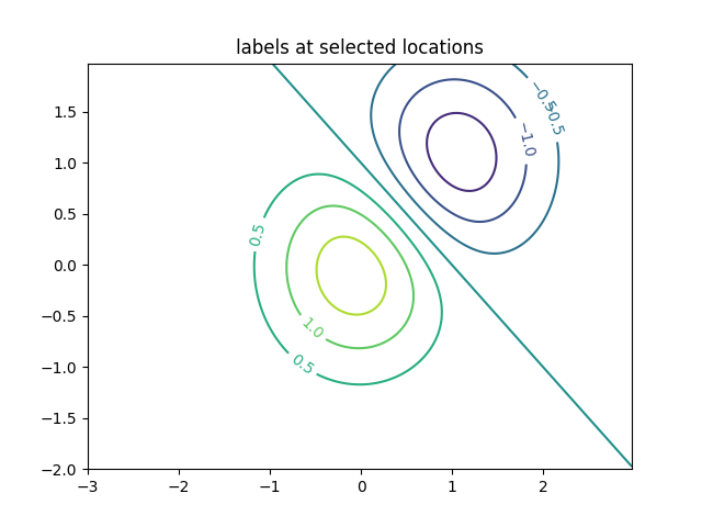
Las etiquetas de contorno se pueden colocar manualmente proporcionando una lista de posiciones (en coordenadas de datos). Consulte Funciones interactivas para la ubicación interactiva.

fig, ax = plt.subplots()
CS = ax.contour(X, Y, Z)
manual_locations = [
    (-1, -1.4), (-0.62, -0.7), (-2, 0.5), (1.7, 1.2), (2.0, 1.4), (2.4, 1.7)]
ax.clabel(CS, inline=True, fontsize=10, manual=manual_locations)
ax.set_title('labels at selected locations')

Text(0.5, 1.0, 'labels at selected locations')

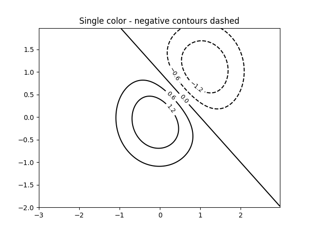
Puede forzar que todos los contornos sean del mismo color.

fig, ax = plt.subplots()
CS = ax.contour(X, Y, Z, 6, colors='k')  # Negative contours default to dashed.
ax.clabel(CS, fontsize=9, inline=True)
ax.set_title('Single color - negative contours dashed')

Un solo color - contornos negativos discontinuos

Text(0.5, 1.0, 'Single color - negative contours dashed')

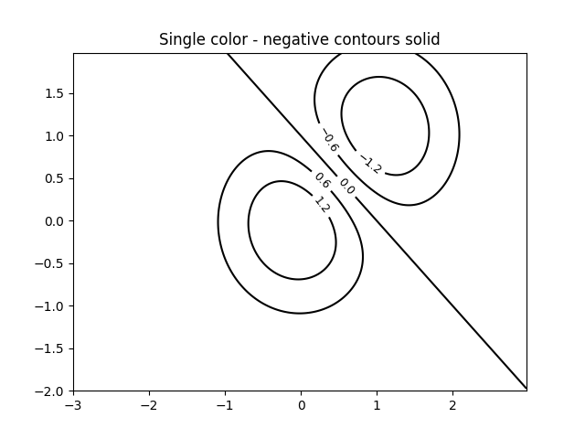
Puede configurar los contornos negativos para que sean sólidos en lugar de discontinuos:

plt.rcParams['contour.negative_linestyle'] = 'solid'
fig, ax = plt.subplots()
CS = ax.contour(X, Y, Z, 6, colors='k')  # Negative contours default to dashed.
ax.clabel(CS, fontsize=9, inline=True)
ax.set_title('Single color - negative contours solid')

Un solo color - contornos negativos sólidos

Text(0.5, 1.0, 'Single color - negative contours solid')

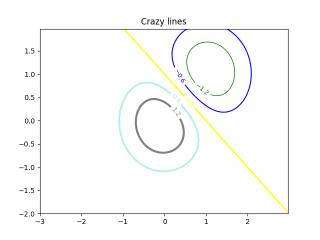
Y puede especificar manualmente los colores del contorno.

fig, ax = plt.subplots()
CS = ax.contour(X, Y, Z, 6,
                linewidths=np.arange(.5, 4, .5),
                colors=('r', 'green', 'blue', (1, 1, 0), '#afeeee', '0.5'),
                )
ax.clabel(CS, fontsize=9, inline=True)
ax.set_title('Crazy lines')

Text(0.5, 1.0, 'Crazy lines')

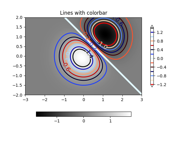
O puede usar un mapa de colores para especificar los colores; el mapa de colores predeterminado se utilizará para las líneas de contorno

fig, ax = plt.subplots()
im = ax.imshow(Z, interpolation='bilinear', origin='lower',
               cmap=cm.gray, extent=(-3, 3, -2, 2))
levels = np.arange(-1.2, 1.6, 0.2)
CS = ax.contour(Z, levels, origin='lower', cmap='flag', extend='both',
                linewidths=2, extent=(-3, 3, -2, 2))

# Thicken the zero contour.
CS.collections[6].set_linewidth(4)

ax.clabel(CS, levels[1::2],  # label every second level
          inline=True, fmt='%1.1f', fontsize=14)

# make a colorbar for the contour lines
CB = fig.colorbar(CS, shrink=0.8)

ax.set_title('Lines with colorbar')

# We can still add a colorbar for the image, too.
CBI = fig.colorbar(im, orientation='horizontal', shrink=0.8)

# This makes the original colorbar look a bit out of place,
# so let's improve its position.

l, b, w, h = ax.get_position().bounds
ll, bb, ww, hh = CB.ax.get_position().bounds
CB.ax.set_position([ll, b + 0.1*h, ww, h*0.8])

plt.show()

Referencias

En este ejemplo se muestra el uso de las siguientes funciones, métodos, clases y módulos:

Tiempo total de ejecución del script: (0 minutos 2,685 segundos)

Galería generada por Sphinx-Gallery