Nota

Haga clic aquí para descargar el código de ejemplo completo

Personalizando Matplotlib con hojas de estilo y rcParams #

Sugerencias para personalizar las propiedades y los estilos predeterminados de Matplotlib.

Hay tres formas de personalizar Matplotlib:

Configuración de rcParams en tiempo de ejecución .

Uso de hojas de estilo .

Cambiando su archivo matplotlibrc .

La configuración de rcParams en tiempo de ejecución tiene prioridad sobre las hojas de estilo, las hojas de estilo tienen prioridad sobre los matplotlibrcarchivos.

Configuración rc en tiempo de ejecución #

Puede cambiar dinámicamente la configuración predeterminada de rc (configuración de tiempo de ejecución) en un script de python o de forma interactiva desde el shell de python. Todas las configuraciones de rc se almacenan en una variable similar a un diccionario llamada matplotlib.rcParams, que es global para el paquete matplotlib. Consulte matplotlib.rcParamspara obtener una lista completa de rcParams configurables. rcParams se puede modificar directamente, por ejemplo:

import numpy as np
import matplotlib.pyplot as plt
import matplotlib as mpl
from cycler import cycler
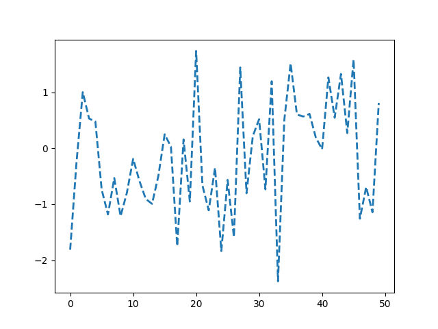
mpl.rcParams['lines.linewidth'] = 2
mpl.rcParams['lines.linestyle'] = '--'
data = np.random.randn(50)
plt.plot(data)

[<matplotlib.lines.Line2D object at 0x7f2cdd6a05b0>]

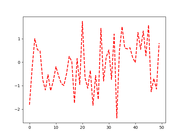
Tenga en cuenta que para cambiar el plotcolor habitual, debe cambiar la propiedad prop_cycle de los ejes :

mpl.rcParams['axes.prop_cycle'] = cycler(color=['r', 'g', 'b', 'y'])
plt.plot(data)  # first color is red

[<matplotlib.lines.Line2D object at 0x7f2cdda41e70>]

Matplotlib también proporciona un par de funciones convenientes para modificar la configuración de rc. matplotlib.rcse puede usar para modificar varias configuraciones en un solo grupo a la vez, usando argumentos de palabras clave:

mpl.rc('lines', linewidth=4, linestyle='-.')
plt.plot(data)

[<matplotlib.lines.Line2D object at 0x7f2cdd6a0b50>]

Configuraciones rc temporales #

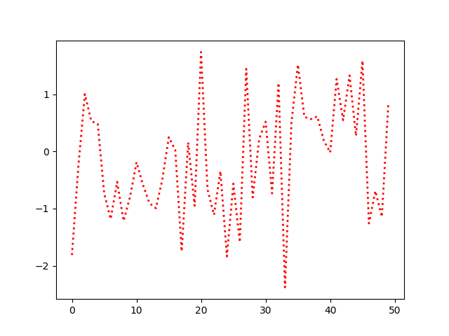
El matplotlib.rcParamsobjeto también se puede cambiar temporalmente usando el matplotlib.rc_contextadministrador de contexto:

with mpl.rc_context({'lines.linewidth': 2, 'lines.linestyle': ':'}):
    plt.plot(data)

matplotlib.rc_contexttambién se puede usar como decorador para modificar los valores predeterminados dentro de una función:

@mpl.rc_context({'lines.linewidth': 3, 'lines.linestyle': '-'})
def plotting_function():
    plt.plot(data)

plotting_function()

matplotlib.rcdefaultsrestaurará la configuración predeterminada estándar de Matplotlib.

Existe cierto grado de validación cuando se establecen los valores de rcParams; consulte matplotlib.rcsetuplos detalles.

Uso de hojas de estilo #

Otra forma de cambiar la apariencia visual de los gráficos es configurar rcParams en una hoja de estilo e importar esa hoja de estilo con matplotlib.style.use. De esta manera, puede cambiar fácilmente entre diferentes estilos simplemente cambiando la hoja de estilo importada. Una hoja de estilo tiene el mismo aspecto que un archivo matplotlibrc , pero en una hoja de estilo solo puede establecer rcParams que estén relacionados con el estilo real de un gráfico. Se ignorarán otros rcParams, como backend . matplotlibrcLos archivos admiten todos los rcParams. La razón detrás de esto es hacer que las hojas de estilo sean portátiles entre diferentes máquinas sin tener que preocuparse por las dependencias que podrían o no estar instaladas en otra máquina. Para obtener una lista completa de rcParams, consulte matplotlib.rcParams. Para obtener una lista de rcParams que se ignoran en las hojas de estilo, consultematplotlib.style.use.

Hay una serie de estilos predefinidos proporcionados por Matplotlib . Por ejemplo, hay un estilo predefinido llamado "ggplot", que emula la estética de ggplot (un popular paquete de trazado para R ). Para usar este estilo, agregue:

plt.style.use('ggplot')

Para listar todos los estilos disponibles, use:

print(plt.style.available)

['Solarize_Light2', '_classic_test_patch', '_mpl-gallery', '_mpl-gallery-nogrid', 'bmh', 'classic', 'dark_background', 'fast', 'fivethirtyeight', 'ggplot', 'grayscale', 'seaborn-v0_8', 'seaborn-v0_8-bright', 'seaborn-v0_8-colorblind', 'seaborn-v0_8-dark', 'seaborn-v0_8-dark-palette', 'seaborn-v0_8-darkgrid', 'seaborn-v0_8-deep', 'seaborn-v0_8-muted', 'seaborn-v0_8-notebook', 'seaborn-v0_8-paper', 'seaborn-v0_8-pastel', 'seaborn-v0_8-poster', 'seaborn-v0_8-talk', 'seaborn-v0_8-ticks', 'seaborn-v0_8-white', 'seaborn-v0_8-whitegrid', 'tableau-colorblind10']

Definiendo tu propio estilo #

Puede crear estilos personalizados y usarlos llamando style.usecon la ruta o URL a la hoja de estilo.

Por ejemplo, es posible que desee crear ./images/presentation.mplstylecon lo siguiente:

axes.titlesize : 24
axes.labelsize : 20
lines.linewidth : 3
lines.markersize : 10
xtick.labelsize : 16
ytick.labelsize : 16

Luego, cuando desee adaptar una trama diseñada para un artículo a una que se vea bien en una presentación, simplemente puede agregar:

>>> import matplotlib.pyplot as plt
>>> plt.style.use('./images/presentation.mplstyle')

Alternativamente, puede dar a conocer su estilo a Matplotlib colocando su <style-name>.mplstylearchivo en mpl_configdir/stylelib. A continuación, puede cargar su hoja de estilo personalizada con una llamada a style.use(<style-name>). Por defecto mpl_configdirdebería ser ~/.config/matplotlib, pero puedes comprobar dónde está el tuyo con matplotlib.get_configdir(); es posible que deba crear este directorio. También puede cambiar el directorio donde Matplotlib busca la carpeta stylelib/ configurando elMPLCONFIGDIRvariable de entorno, consulte la configuración de matplotlib y las ubicaciones del directorio de caché .

Tenga en cuenta que una hoja de estilo personalizada mpl_configdir/stylelibanulará una hoja de estilo definida por Matplotlib si los estilos tienen el mismo nombre.

Una vez que su <style-name>.mplstylearchivo esté en el lugar apropiado mpl_configdir, puede especificar su estilo con:

>>> import matplotlib.pyplot as plt
>>> plt.style.use(<style-name>)

Estilos de composición #

Las hojas de estilo están diseñadas para componerse juntas. Por lo tanto, puede tener una hoja de estilo que personalice los colores y una hoja de estilo independiente que altere los tamaños de los elementos para las presentaciones. Estos estilos se pueden combinar fácilmente pasando una lista de estilos:

>>> import matplotlib.pyplot as plt
>>> plt.style.use(['dark_background', 'presentation'])

Tenga en cuenta que los estilos más a la derecha sobrescribirán los valores que ya están definidos por los estilos de la izquierda.

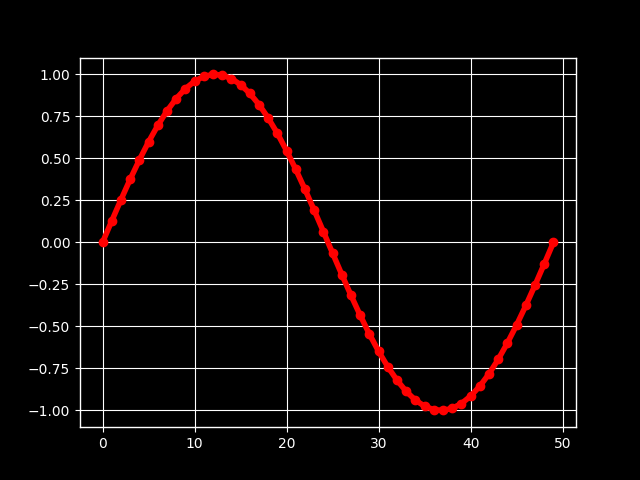
Estilo temporal #

Si solo desea usar un estilo para un bloque de código específico pero no desea cambiar el estilo global, el paquete de estilo proporciona un administrador de contexto para limitar sus cambios a un ámbito específico. Para aislar sus cambios de estilo, puede escribir algo como lo siguiente:

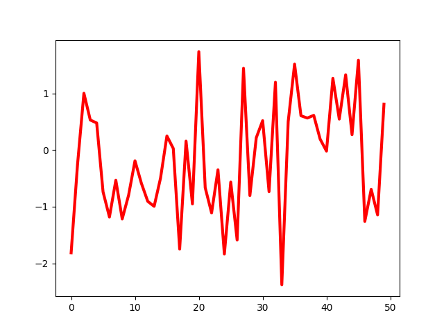
with plt.style.context('dark_background'):
    plt.plot(np.sin(np.linspace(0, 2 * np.pi)), 'r-o')
plt.show()

El `matplotlibrc`archivo #

Matplotlib usa matplotlibrcarchivos de configuración para personalizar todo tipo de propiedades, que llamamos 'configuración rc' o 'parámetros rc'. Puede controlar los valores predeterminados de casi todas las propiedades en Matplotlib: tamaño de figura y DPI, ancho de línea, color y estilo, ejes, propiedades de eje y cuadrícula, propiedades de texto y fuente, etc. Se matplotlibrclee al inicio para configurar Matplotlib. Matplotlib busca matplotlibrcen cuatro ubicaciones, en el siguiente orden:

matplotlibrcen el directorio de trabajo actual, generalmente utilizado para personalizaciones específicas que no desea aplicar en ningún otro lugar.
$MATPLOTLIBRCsi es un archivo, de lo contrario $MATPLOTLIBRC/matplotlibrc.
A continuación, se ve en un lugar específico del usuario, según su plataforma:
- En Linux y FreeBSD, busca en .config/matplotlib/matplotlibrc(o $XDG_CONFIG_HOME/matplotlib/matplotlibrc) si ha personalizado su entorno.
- En otras plataformas, se ve en .matplotlib/matplotlibrc.
Consulte la configuración de matplotlib y las ubicaciones del directorio de caché .
INSTALL/matplotlib/mpl-data/matplotlibrc, donde INSTALLes algo así como /usr/lib/python3.9/site-packagesen Linux, y tal vez C:\Python39\Lib\site-packagesen Windows. Cada vez que instale matplotlib, este archivo se sobrescribirá, por lo que si desea que se guarden sus personalizaciones, mueva este archivo a su directorio matplotlib específico del usuario.

matplotlibrcUna vez que se ha encontrado un archivo, no buscará ninguna de las otras rutas. Cuando se asigna una hoja de estilo con style.use('<path>/<style-name>.mplstyle'), la configuración especificada en la hoja de estilo tiene prioridad sobre la configuración del matplotlibrcarchivo.

matplotlibrcPara mostrar desde dónde se cargó el archivo actualmente activo , se puede hacer lo siguiente:

>>> import matplotlib
>>> matplotlib.matplotlib_fname()
'/home/foo/.config/matplotlib/matplotlibrc'

Vea a continuación un archivo matplotlibrc de muestra y vea matplotlib.rcParamsuna lista completa de rcParams configurables.

`matplotlibrc`El archivo predeterminado #

#### MATPLOTLIBRC FORMAT

## NOTE FOR END USERS: DO NOT EDIT THIS FILE!
##
## This is a sample Matplotlib configuration file - you can find a copy
## of it on your system in site-packages/matplotlib/mpl-data/matplotlibrc
## (relative to your Python installation location).
## DO NOT EDIT IT!
##
## If you wish to change your default style, copy this file to one of the
## following locations:
##     Unix/Linux:
##         $HOME/.config/matplotlib/matplotlibrc OR
##         $XDG_CONFIG_HOME/matplotlib/matplotlibrc (if $XDG_CONFIG_HOME is set)
##     Other platforms:
##         $HOME/.matplotlib/matplotlibrc
## and edit that copy.
##
## See https://matplotlib.org/stable/tutorials/introductory/customizing.html#customizing-with-matplotlibrc-files
## for more details on the paths which are checked for the configuration file.
##
## Blank lines, or lines starting with a comment symbol, are ignored, as are
## trailing comments.  Other lines must have the format:
##     key: val  # optional comment
##
## Formatting: Use PEP8-like style (as enforced in the rest of the codebase).
## All lines start with an additional '#', so that removing all leading '#'s
## yields a valid style file.
##
## Colors: for the color values below, you can either use
##     - a Matplotlib color string, such as r, k, or b
##     - an RGB tuple, such as (1.0, 0.5, 0.0)
##     - a double-quoted hex string, such as "#ff00ff".
##       The unquoted string ff00ff is also supported for backward
##       compatibility, but is discouraged.
##     - a scalar grayscale intensity such as 0.75
##     - a legal html color name, e.g., red, blue, darkslategray
##
## String values may optionally be enclosed in double quotes, which allows
## using the comment character # in the string.
##
## This file (and other style files) must be encoded as utf-8.
##
## Matplotlib configuration are currently divided into following parts:
##     - BACKENDS
##     - LINES
##     - PATCHES
##     - HATCHES
##     - BOXPLOT
##     - FONT
##     - TEXT
##     - LaTeX
##     - AXES
##     - DATES
##     - TICKS
##     - GRIDS
##     - LEGEND
##     - FIGURE
##     - IMAGES
##     - CONTOUR PLOTS
##     - ERRORBAR PLOTS
##     - HISTOGRAM PLOTS
##     - SCATTER PLOTS
##     - AGG RENDERING
##     - PATHS
##     - SAVING FIGURES
##     - INTERACTIVE KEYMAPS
##     - ANIMATION

##### CONFIGURATION BEGINS HERE


## ***************************************************************************
## * BACKENDS                                                                *
## ***************************************************************************
## The default backend.  If you omit this parameter, the first working
## backend from the following list is used:
##     MacOSX QtAgg Gtk4Agg Gtk3Agg TkAgg WxAgg Agg
## Other choices include:
##     QtCairo GTK4Cairo GTK3Cairo TkCairo WxCairo Cairo
##     Qt5Agg Qt5Cairo Wx  # deprecated.
##     PS PDF SVG Template
## You can also deploy your own backend outside of Matplotlib by referring to
## the module name (which must be in the PYTHONPATH) as 'module://my_backend'.
##backend: Agg

## The port to use for the web server in the WebAgg backend.
#webagg.port: 8988

## The address on which the WebAgg web server should be reachable
#webagg.address: 127.0.0.1

## If webagg.port is unavailable, a number of other random ports will
## be tried until one that is available is found.
#webagg.port_retries: 50

## When True, open the web browser to the plot that is shown
#webagg.open_in_browser: True

## If you are running pyplot inside a GUI and your backend choice
## conflicts, we will automatically try to find a compatible one for
## you if backend_fallback is True
#backend_fallback: True

#interactive: False
#toolbar:     toolbar2  # {None, toolbar2, toolmanager}
#timezone:    UTC       # a pytz timezone string, e.g., US/Central or Europe/Paris


## ***************************************************************************
## * LINES                                                                   *
## ***************************************************************************
## See https://matplotlib.org/api/artist_api.html#module-matplotlib.lines
## for more information on line properties.
#lines.linewidth: 1.5               # line width in points
#lines.linestyle: -                 # solid line
#lines.color:     C0                # has no affect on plot(); see axes.prop_cycle
#lines.marker:          None        # the default marker
#lines.markerfacecolor: auto        # the default marker face color
#lines.markeredgecolor: auto        # the default marker edge color
#lines.markeredgewidth: 1.0         # the line width around the marker symbol
#lines.markersize:      6           # marker size, in points
#lines.dash_joinstyle:  round       # {miter, round, bevel}
#lines.dash_capstyle:   butt        # {butt, round, projecting}
#lines.solid_joinstyle: round       # {miter, round, bevel}
#lines.solid_capstyle:  projecting  # {butt, round, projecting}
#lines.antialiased: True            # render lines in antialiased (no jaggies)

## The three standard dash patterns.  These are scaled by the linewidth.
#lines.dashed_pattern: 3.7, 1.6
#lines.dashdot_pattern: 6.4, 1.6, 1, 1.6
#lines.dotted_pattern: 1, 1.65
#lines.scale_dashes: True

#markers.fillstyle: full  # {full, left, right, bottom, top, none}

#pcolor.shading: auto
#pcolormesh.snap: True  # Whether to snap the mesh to pixel boundaries. This is
                        # provided solely to allow old test images to remain
                        # unchanged. Set to False to obtain the previous behavior.

## ***************************************************************************
## * PATCHES                                                                 *
## ***************************************************************************
## Patches are graphical objects that fill 2D space, like polygons or circles.
## See https://matplotlib.org/api/artist_api.html#module-matplotlib.patches
## for more information on patch properties.
#patch.linewidth:       1.0    # edge width in points.
#patch.facecolor:       C0
#patch.edgecolor:       black  # if forced, or patch is not filled
#patch.force_edgecolor: False  # True to always use edgecolor
#patch.antialiased:     True   # render patches in antialiased (no jaggies)


## ***************************************************************************
## * HATCHES                                                                 *
## ***************************************************************************
#hatch.color:     black
#hatch.linewidth: 1.0


## ***************************************************************************
## * BOXPLOT                                                                 *
## ***************************************************************************
#boxplot.notch:       False
#boxplot.vertical:    True
#boxplot.whiskers:    1.5
#boxplot.bootstrap:   None
#boxplot.patchartist: False
#boxplot.showmeans:   False
#boxplot.showcaps:    True
#boxplot.showbox:     True
#boxplot.showfliers:  True
#boxplot.meanline:    False

#boxplot.flierprops.color:           black
#boxplot.flierprops.marker:          o
#boxplot.flierprops.markerfacecolor: none
#boxplot.flierprops.markeredgecolor: black
#boxplot.flierprops.markeredgewidth: 1.0
#boxplot.flierprops.markersize:      6
#boxplot.flierprops.linestyle:       none
#boxplot.flierprops.linewidth:       1.0

#boxplot.boxprops.color:     black
#boxplot.boxprops.linewidth: 1.0
#boxplot.boxprops.linestyle: -

#boxplot.whiskerprops.color:     black
#boxplot.whiskerprops.linewidth: 1.0
#boxplot.whiskerprops.linestyle: -

#boxplot.capprops.color:     black
#boxplot.capprops.linewidth: 1.0
#boxplot.capprops.linestyle: -

#boxplot.medianprops.color:     C1
#boxplot.medianprops.linewidth: 1.0
#boxplot.medianprops.linestyle: -

#boxplot.meanprops.color:           C2
#boxplot.meanprops.marker:          ^
#boxplot.meanprops.markerfacecolor: C2
#boxplot.meanprops.markeredgecolor: C2
#boxplot.meanprops.markersize:       6
#boxplot.meanprops.linestyle:       --
#boxplot.meanprops.linewidth:       1.0


## ***************************************************************************
## * FONT                                                                    *
## ***************************************************************************
## The font properties used by `text.Text`.
## See https://matplotlib.org/api/font_manager_api.html for more information
## on font properties.  The 6 font properties used for font matching are
## given below with their default values.
##
## The font.family property can take either a single or multiple entries of any
## combination of concrete font names (not supported when rendering text with
## usetex) or the following five generic values:
##     - 'serif' (e.g., Times),
##     - 'sans-serif' (e.g., Helvetica),
##     - 'cursive' (e.g., Zapf-Chancery),
##     - 'fantasy' (e.g., Western), and
##     - 'monospace' (e.g., Courier).
## Each of these values has a corresponding default list of font names
## (font.serif, etc.); the first available font in the list is used.  Note that
## for font.serif, font.sans-serif, and font.monospace, the first element of
## the list (a DejaVu font) will always be used because DejaVu is shipped with
## Matplotlib and is thus guaranteed to be available; the other entries are
## left as examples of other possible values.
##
## The font.style property has three values: normal (or roman), italic
## or oblique.  The oblique style will be used for italic, if it is not
## present.
##
## The font.variant property has two values: normal or small-caps.  For
## TrueType fonts, which are scalable fonts, small-caps is equivalent
## to using a font size of 'smaller', or about 83%% of the current font
## size.
##
## The font.weight property has effectively 13 values: normal, bold,
## bolder, lighter, 100, 200, 300, ..., 900.  Normal is the same as
## 400, and bold is 700.  bolder and lighter are relative values with
## respect to the current weight.
##
## The font.stretch property has 11 values: ultra-condensed,
## extra-condensed, condensed, semi-condensed, normal, semi-expanded,
## expanded, extra-expanded, ultra-expanded, wider, and narrower.  This
## property is not currently implemented.
##
## The font.size property is the default font size for text, given in points.
## 10 pt is the standard value.
##
## Note that font.size controls default text sizes.  To configure
## special text sizes tick labels, axes, labels, title, etc., see the rc
## settings for axes and ticks.  Special text sizes can be defined
## relative to font.size, using the following values: xx-small, x-small,
## small, medium, large, x-large, xx-large, larger, or smaller

#font.family:  sans-serif
#font.style:   normal
#font.variant: normal
#font.weight:  normal
#font.stretch: normal
#font.size:    10.0

#font.serif:      DejaVu Serif, Bitstream Vera Serif, Computer Modern Roman, New Century Schoolbook, Century Schoolbook L, Utopia, ITC Bookman, Bookman, Nimbus Roman No9 L, Times New Roman, Times, Palatino, Charter, serif
#font.sans-serif: DejaVu Sans, Bitstream Vera Sans, Computer Modern Sans Serif, Lucida Grande, Verdana, Geneva, Lucid, Arial, Helvetica, Avant Garde, sans-serif
#font.cursive:    Apple Chancery, Textile, Zapf Chancery, Sand, Script MT, Felipa, Comic Neue, Comic Sans MS, cursive
#font.fantasy:    Chicago, Charcoal, Impact, Western, Humor Sans, xkcd, fantasy
#font.monospace:  DejaVu Sans Mono, Bitstream Vera Sans Mono, Computer Modern Typewriter, Andale Mono, Nimbus Mono L, Courier New, Courier, Fixed, Terminal, monospace


## ***************************************************************************
## * TEXT                                                                    *
## ***************************************************************************
## The text properties used by `text.Text`.
## See https://matplotlib.org/api/artist_api.html#module-matplotlib.text
## for more information on text properties
#text.color: black

## FreeType hinting flag ("foo" corresponds to FT_LOAD_FOO); may be one of the
## following (Proprietary Matplotlib-specific synonyms are given in parentheses,
## but their use is discouraged):
## - default: Use the font's native hinter if possible, else FreeType's auto-hinter.
##            ("either" is a synonym).
## - no_autohint: Use the font's native hinter if possible, else don't hint.
##                ("native" is a synonym.)
## - force_autohint: Use FreeType's auto-hinter.  ("auto" is a synonym.)
## - no_hinting: Disable hinting.  ("none" is a synonym.)
#text.hinting: force_autohint

#text.hinting_factor: 8  # Specifies the amount of softness for hinting in the
                         # horizontal direction.  A value of 1 will hint to full
                         # pixels.  A value of 2 will hint to half pixels etc.
#text.kerning_factor: 0  # Specifies the scaling factor for kerning values.  This
                         # is provided solely to allow old test images to remain
                         # unchanged.  Set to 6 to obtain previous behavior.
                         # Values  other than 0 or 6 have no defined meaning.
#text.antialiased: True  # If True (default), the text will be antialiased.
                         # This only affects raster outputs.
#text.parse_math: True  # Use mathtext if there is an even number of unescaped
                        # dollar signs.


## ***************************************************************************
## * LaTeX                                                                   *
## ***************************************************************************
## For more information on LaTeX properties, see
## https://matplotlib.org/tutorials/text/usetex.html
#text.usetex: False  # use latex for all text handling. The following fonts
                     # are supported through the usual rc parameter settings:
                     # new century schoolbook, bookman, times, palatino,
                     # zapf chancery, charter, serif, sans-serif, helvetica,
                     # avant garde, courier, monospace, computer modern roman,
                     # computer modern sans serif, computer modern typewriter
#text.latex.preamble:   # IMPROPER USE OF THIS FEATURE WILL LEAD TO LATEX FAILURES
                        # AND IS THEREFORE UNSUPPORTED. PLEASE DO NOT ASK FOR HELP
                        # IF THIS FEATURE DOES NOT DO WHAT YOU EXPECT IT TO.
                        # text.latex.preamble is a single line of LaTeX code that
                        # will be passed on to the LaTeX system. It may contain
                        # any code that is valid for the LaTeX "preamble", i.e.
                        # between the "\documentclass" and "\begin{document}"
                        # statements.
                        # Note that it has to be put on a single line, which may
                        # become quite long.
                        # The following packages are always loaded with usetex,
                        # so beware of package collisions:
                        #   geometry, inputenc, type1cm.
                        # PostScript (PSNFSS) font packages may also be
                        # loaded, depending on your font settings.

## The following settings allow you to select the fonts in math mode.
#mathtext.fontset: dejavusans  # Should be 'dejavusans' (default),
                               # 'dejavuserif', 'cm' (Computer Modern), 'stix',
                               # 'stixsans' or 'custom' (unsupported, may go
                               # away in the future)
## "mathtext.fontset: custom" is defined by the mathtext.bf, .cal, .it, ...
## settings which map a TeX font name to a fontconfig font pattern.  (These
## settings are not used for other font sets.)
#mathtext.bf:  sans:bold
#mathtext.cal: cursive
#mathtext.it:  sans:italic
#mathtext.rm:  sans
#mathtext.sf:  sans
#mathtext.tt:  monospace
#mathtext.fallback: cm  # Select fallback font from ['cm' (Computer Modern), 'stix'
                        # 'stixsans'] when a symbol can not be found in one of the
                        # custom math fonts. Select 'None' to not perform fallback
                        # and replace the missing character by a dummy symbol.
#mathtext.default: it  # The default font to use for math.
                       # Can be any of the LaTeX font names, including
                       # the special name "regular" for the same font
                       # used in regular text.


## ***************************************************************************
## * AXES                                                                    *
## ***************************************************************************
## Following are default face and edge colors, default tick sizes,
## default font sizes for tick labels, and so on.  See
## https://matplotlib.org/api/axes_api.html#module-matplotlib.axes
#axes.facecolor:     white   # axes background color
#axes.edgecolor:     black   # axes edge color
#axes.linewidth:     0.8     # edge line width
#axes.grid:          False   # display grid or not
#axes.grid.axis:     both    # which axis the grid should apply to
#axes.grid.which:    major   # grid lines at {major, minor, both} ticks
#axes.titlelocation: center  # alignment of the title: {left, right, center}
#axes.titlesize:     large   # font size of the axes title
#axes.titleweight:   normal  # font weight of title
#axes.titlecolor:    auto    # color of the axes title, auto falls back to
                             # text.color as default value
#axes.titley:        None    # position title (axes relative units).  None implies auto
#axes.titlepad:      6.0     # pad between axes and title in points
#axes.labelsize:     medium  # font size of the x and y labels
#axes.labelpad:      4.0     # space between label and axis
#axes.labelweight:   normal  # weight of the x and y labels
#axes.labelcolor:    black
#axes.axisbelow:     line    # draw axis gridlines and ticks:
                             #     - below patches (True)
                             #     - above patches but below lines ('line')
                             #     - above all (False)

#axes.formatter.limits: -5, 6  # use scientific notation if log10
                               # of the axis range is smaller than the
                               # first or larger than the second
#axes.formatter.use_locale: False  # When True, format tick labels
                                   # according to the user's locale.
                                   # For example, use ',' as a decimal
                                   # separator in the fr_FR locale.
#axes.formatter.use_mathtext: False  # When True, use mathtext for scientific
                                     # notation.
#axes.formatter.min_exponent: 0  # minimum exponent to format in scientific notation
#axes.formatter.useoffset: True  # If True, the tick label formatter
                                 # will default to labeling ticks relative
                                 # to an offset when the data range is
                                 # small compared to the minimum absolute
                                 # value of the data.
#axes.formatter.offset_threshold: 4  # When useoffset is True, the offset
                                     # will be used when it can remove
                                     # at least this number of significant
                                     # digits from tick labels.

#axes.spines.left:   True  # display axis spines
#axes.spines.bottom: True
#axes.spines.top:    True
#axes.spines.right:  True

#axes.unicode_minus: True  # use Unicode for the minus symbol rather than hyphen.  See
                           # https://en.wikipedia.org/wiki/Plus_and_minus_signs#Character_codes
#axes.prop_cycle: cycler('color', ['1f77b4', 'ff7f0e', '2ca02c', 'd62728', '9467bd', '8c564b', 'e377c2', '7f7f7f', 'bcbd22', '17becf'])
                  # color cycle for plot lines as list of string color specs:
                  # single letter, long name, or web-style hex
                  # As opposed to all other parameters in this file, the color
                  # values must be enclosed in quotes for this parameter,
                  # e.g. '1f77b4', instead of 1f77b4.
                  # See also https://matplotlib.org/tutorials/intermediate/color_cycle.html
                  # for more details on prop_cycle usage.
#axes.xmargin:   .05  # x margin.  See `axes.Axes.margins`
#axes.ymargin:   .05  # y margin.  See `axes.Axes.margins`
#axes.zmargin:   .05  # z margin.  See `axes.Axes.margins`
#axes.autolimit_mode: data  # If "data", use axes.xmargin and axes.ymargin as is.
                            # If "round_numbers", after application of margins, axis
                            # limits are further expanded to the nearest "round" number.
#polaraxes.grid: True  # display grid on polar axes
#axes3d.grid:    True  # display grid on 3D axes


## ***************************************************************************
## * AXIS                                                                    *
## ***************************************************************************
#xaxis.labellocation: center  # alignment of the xaxis label: {left, right, center}
#yaxis.labellocation: center  # alignment of the yaxis label: {bottom, top, center}


## ***************************************************************************
## * DATES                                                                   *
## ***************************************************************************
## These control the default format strings used in AutoDateFormatter.
## Any valid format datetime format string can be used (see the python
## `datetime` for details).  For example, by using:
##     - '%%x' will use the locale date representation
##     - '%%X' will use the locale time representation
##     - '%%c' will use the full locale datetime representation
## These values map to the scales:
##     {'year': 365, 'month': 30, 'day': 1, 'hour': 1/24, 'minute': 1 / (24 * 60)}

#date.autoformatter.year:        %Y
#date.autoformatter.month:       %Y-%m
#date.autoformatter.day:         %Y-%m-%d
#date.autoformatter.hour:        %m-%d %H
#date.autoformatter.minute:      %d %H:%M
#date.autoformatter.second:      %H:%M:%S
#date.autoformatter.microsecond: %M:%S.%f
## The reference date for Matplotlib's internal date representation
## See https://matplotlib.org/examples/ticks_and_spines/date_precision_and_epochs.py
#date.epoch: 1970-01-01T00:00:00
## 'auto', 'concise':
#date.converter:                  auto
## For auto converter whether to use interval_multiples:
#date.interval_multiples:         True

## ***************************************************************************
## * TICKS                                                                   *
## ***************************************************************************
## See https://matplotlib.org/api/axis_api.html#matplotlib.axis.Tick
#xtick.top:           False   # draw ticks on the top side
#xtick.bottom:        True    # draw ticks on the bottom side
#xtick.labeltop:      False   # draw label on the top
#xtick.labelbottom:   True    # draw label on the bottom
#xtick.major.size:    3.5     # major tick size in points
#xtick.minor.size:    2       # minor tick size in points
#xtick.major.width:   0.8     # major tick width in points
#xtick.minor.width:   0.6     # minor tick width in points
#xtick.major.pad:     3.5     # distance to major tick label in points
#xtick.minor.pad:     3.4     # distance to the minor tick label in points
#xtick.color:         black   # color of the ticks
#xtick.labelcolor:    inherit # color of the tick labels or inherit from xtick.color
#xtick.labelsize:     medium  # font size of the tick labels
#xtick.direction:     out     # direction: {in, out, inout}
#xtick.minor.visible: False   # visibility of minor ticks on x-axis
#xtick.major.top:     True    # draw x axis top major ticks
#xtick.major.bottom:  True    # draw x axis bottom major ticks
#xtick.minor.top:     True    # draw x axis top minor ticks
#xtick.minor.bottom:  True    # draw x axis bottom minor ticks
#xtick.alignment:     center  # alignment of xticks

#ytick.left:          True    # draw ticks on the left side
#ytick.right:         False   # draw ticks on the right side
#ytick.labelleft:     True    # draw tick labels on the left side
#ytick.labelright:    False   # draw tick labels on the right side
#ytick.major.size:    3.5     # major tick size in points
#ytick.minor.size:    2       # minor tick size in points
#ytick.major.width:   0.8     # major tick width in points
#ytick.minor.width:   0.6     # minor tick width in points
#ytick.major.pad:     3.5     # distance to major tick label in points
#ytick.minor.pad:     3.4     # distance to the minor tick label in points
#ytick.color:         black   # color of the ticks
#ytick.labelcolor:    inherit # color of the tick labels or inherit from ytick.color
#ytick.labelsize:     medium  # font size of the tick labels
#ytick.direction:     out     # direction: {in, out, inout}
#ytick.minor.visible: False   # visibility of minor ticks on y-axis
#ytick.major.left:    True    # draw y axis left major ticks
#ytick.major.right:   True    # draw y axis right major ticks
#ytick.minor.left:    True    # draw y axis left minor ticks
#ytick.minor.right:   True    # draw y axis right minor ticks
#ytick.alignment:     center_baseline  # alignment of yticks


## ***************************************************************************
## * GRIDS                                                                   *
## ***************************************************************************
#grid.color:     "#b0b0b0"  # grid color
#grid.linestyle: -          # solid
#grid.linewidth: 0.8        # in points
#grid.alpha:     1.0        # transparency, between 0.0 and 1.0


## ***************************************************************************
## * LEGEND                                                                  *
## ***************************************************************************
#legend.loc:           best
#legend.frameon:       True     # if True, draw the legend on a background patch
#legend.framealpha:    0.8      # legend patch transparency
#legend.facecolor:     inherit  # inherit from axes.facecolor; or color spec
#legend.edgecolor:     0.8      # background patch boundary color
#legend.fancybox:      True     # if True, use a rounded box for the
                                # legend background, else a rectangle
#legend.shadow:        False    # if True, give background a shadow effect
#legend.numpoints:     1        # the number of marker points in the legend line
#legend.scatterpoints: 1        # number of scatter points
#legend.markerscale:   1.0      # the relative size of legend markers vs. original
#legend.fontsize:      medium
#legend.labelcolor:    None
#legend.title_fontsize: None    # None sets to the same as the default axes.

## Dimensions as fraction of font size:
#legend.borderpad:     0.4  # border whitespace
#legend.labelspacing:  0.5  # the vertical space between the legend entries
#legend.handlelength:  2.0  # the length of the legend lines
#legend.handleheight:  0.7  # the height of the legend handle
#legend.handletextpad: 0.8  # the space between the legend line and legend text
#legend.borderaxespad: 0.5  # the border between the axes and legend edge
#legend.columnspacing: 2.0  # column separation


## ***************************************************************************
## * FIGURE                                                                  *
## ***************************************************************************
## See https://matplotlib.org/api/figure_api.html#matplotlib.figure.Figure
#figure.titlesize:   large     # size of the figure title (``Figure.suptitle()``)
#figure.titleweight: normal    # weight of the figure title
#figure.labelsize:   large     # size of the figure label (``Figure.sup[x|y]label()``)
#figure.labelweight: normal    # weight of the figure label
#figure.figsize:     6.4, 4.8  # figure size in inches
#figure.dpi:         100       # figure dots per inch
#figure.facecolor:   white     # figure face color
#figure.edgecolor:   white     # figure edge color
#figure.frameon:     True      # enable figure frame
#figure.max_open_warning: 20   # The maximum number of figures to open through
                               # the pyplot interface before emitting a warning.
                               # If less than one this feature is disabled.
#figure.raise_window : True    # Raise the GUI window to front when show() is called.

## The figure subplot parameters.  All dimensions are a fraction of the figure width and height.
#figure.subplot.left:   0.125  # the left side of the subplots of the figure
#figure.subplot.right:  0.9    # the right side of the subplots of the figure
#figure.subplot.bottom: 0.11   # the bottom of the subplots of the figure
#figure.subplot.top:    0.88   # the top of the subplots of the figure
#figure.subplot.wspace: 0.2    # the amount of width reserved for space between subplots,
                               # expressed as a fraction of the average axis width
#figure.subplot.hspace: 0.2    # the amount of height reserved for space between subplots,
                               # expressed as a fraction of the average axis height

## Figure layout
#figure.autolayout: False  # When True, automatically adjust subplot
                           # parameters to make the plot fit the figure
                           # using `tight_layout`
#figure.constrained_layout.use: False  # When True, automatically make plot
                                       # elements fit on the figure. (Not
                                       # compatible with `autolayout`, above).
#figure.constrained_layout.h_pad:  0.04167  # Padding around axes objects. Float representing
#figure.constrained_layout.w_pad:  0.04167  # inches. Default is 3/72 inches (3 points)
#figure.constrained_layout.hspace: 0.02     # Space between subplot groups. Float representing
#figure.constrained_layout.wspace: 0.02     # a fraction of the subplot widths being separated.


## ***************************************************************************
## * IMAGES                                                                  *
## ***************************************************************************
#image.aspect:          equal        # {equal, auto} or a number
#image.interpolation:   antialiased  # see help(imshow) for options
#image.cmap:            viridis      # A colormap name (plasma, magma, etc.)
#image.lut:             256          # the size of the colormap lookup table
#image.origin:          upper        # {lower, upper}
#image.resample:        True
#image.composite_image: True  # When True, all the images on a set of axes are
                              # combined into a single composite image before
                              # saving a figure as a vector graphics file,
                              # such as a PDF.


## ***************************************************************************
## * CONTOUR PLOTS                                                           *
## ***************************************************************************
#contour.negative_linestyle: dashed  # string or on-off ink sequence
#contour.corner_mask:        True    # {True, False}
#contour.linewidth:          None    # {float, None} Size of the contour line
                                     # widths. If set to None, it falls back to
                                     # `line.linewidth`.
#contour.algorithm:          mpl2014 # {mpl2005, mpl2014, serial, threaded}


## ***************************************************************************
## * ERRORBAR PLOTS                                                          *
## ***************************************************************************
#errorbar.capsize: 0  # length of end cap on error bars in pixels


## ***************************************************************************
## * HISTOGRAM PLOTS                                                         *
## ***************************************************************************
#hist.bins: 10  # The default number of histogram bins or 'auto'.


## ***************************************************************************
## * SCATTER PLOTS                                                           *
## ***************************************************************************
#scatter.marker: o         # The default marker type for scatter plots.
#scatter.edgecolors: face  # The default edge colors for scatter plots.


## ***************************************************************************
## * AGG RENDERING                                                           *
## ***************************************************************************
## Warning: experimental, 2008/10/10
#agg.path.chunksize: 0  # 0 to disable; values in the range
                        # 10000 to 100000 can improve speed slightly
                        # and prevent an Agg rendering failure
                        # when plotting very large data sets,
                        # especially if they are very gappy.
                        # It may cause minor artifacts, though.
                        # A value of 20000 is probably a good
                        # starting point.


## ***************************************************************************
## * PATHS                                                                   *
## ***************************************************************************
#path.simplify: True  # When True, simplify paths by removing "invisible"
                      # points to reduce file size and increase rendering
                      # speed
#path.simplify_threshold: 0.111111111111  # The threshold of similarity below
                                          # which vertices will be removed in
                                          # the simplification process.
#path.snap: True  # When True, rectilinear axis-aligned paths will be snapped
                  # to the nearest pixel when certain criteria are met.
                  # When False, paths will never be snapped.
#path.sketch: None  # May be None, or a 3-tuple of the form:
                    # (scale, length, randomness).
                    #     - *scale* is the amplitude of the wiggle
                    #         perpendicular to the line (in pixels).
                    #     - *length* is the length of the wiggle along the
                    #         line (in pixels).
                    #     - *randomness* is the factor by which the length is
                    #         randomly scaled.
#path.effects:


## ***************************************************************************
## * SAVING FIGURES                                                          *
## ***************************************************************************
## The default savefig parameters can be different from the display parameters
## e.g., you may want a higher resolution, or to make the figure
## background white
#savefig.dpi:       figure      # figure dots per inch or 'figure'
#savefig.facecolor: auto        # figure face color when saving
#savefig.edgecolor: auto        # figure edge color when saving
#savefig.format:    png         # {png, ps, pdf, svg}
#savefig.bbox:      standard    # {tight, standard}
                                # 'tight' is incompatible with pipe-based animation
                                # backends (e.g. 'ffmpeg') but will work with those
                                # based on temporary files (e.g. 'ffmpeg_file')
#savefig.pad_inches:  0.1       # padding to be used, when bbox is set to 'tight'
#savefig.directory:   ~         # default directory in savefig dialog, gets updated after
                                # interactive saves, unless set to the empty string (i.e.
                                # the current directory); use '.' to start at the current
                                # directory but update after interactive saves
#savefig.transparent: False     # whether figures are saved with a transparent
                                # background by default
#savefig.orientation: portrait  # orientation of saved figure, for PostScript output only

### tk backend params
#tk.window_focus:   False  # Maintain shell focus for TkAgg

### ps backend params
#ps.papersize:      letter  # {auto, letter, legal, ledger, A0-A10, B0-B10}
#ps.useafm:         False   # use of AFM fonts, results in small files
#ps.usedistiller:   False   # {ghostscript, xpdf, None}
                            # Experimental: may produce smaller files.
                            # xpdf intended for production of publication quality files,
                            # but requires ghostscript, xpdf and ps2eps
#ps.distiller.res:  6000    # dpi
#ps.fonttype:       3       # Output Type 3 (Type3) or Type 42 (TrueType)

### PDF backend params
#pdf.compression:    6  # integer from 0 to 9
                        # 0 disables compression (good for debugging)
#pdf.fonttype:       3  # Output Type 3 (Type3) or Type 42 (TrueType)
#pdf.use14corefonts: False
#pdf.inheritcolor:   False

### SVG backend params
#svg.image_inline: True  # Write raster image data directly into the SVG file
#svg.fonttype: path      # How to handle SVG fonts:
                         #     path: Embed characters as paths -- supported
                         #           by most SVG renderers
                         #     None: Assume fonts are installed on the
                         #           machine where the SVG will be viewed.
#svg.hashsalt: None      # If not None, use this string as hash salt instead of uuid4

### pgf parameter
## See https://matplotlib.org/tutorials/text/pgf.html for more information.
#pgf.rcfonts: True
#pgf.preamble:  # See text.latex.preamble for documentation
#pgf.texsystem: xelatex

### docstring params
#docstring.hardcopy: False  # set this when you want to generate hardcopy docstring


## ***************************************************************************
## * INTERACTIVE KEYMAPS                                                     *
## ***************************************************************************
## Event keys to interact with figures/plots via keyboard.
## See https://matplotlib.org/stable/users/explain/interactive.html for more
## details on interactive navigation.  Customize these settings according to
## your needs. Leave the field(s) empty if you don't need a key-map. (i.e.,
## fullscreen : '')
#keymap.fullscreen: f, ctrl+f   # toggling
#keymap.home: h, r, home        # home or reset mnemonic
#keymap.back: left, c, backspace, MouseButton.BACK  # forward / backward keys
#keymap.forward: right, v, MouseButton.FORWARD      # for quick navigation
#keymap.pan: p                  # pan mnemonic
#keymap.zoom: o                 # zoom mnemonic
#keymap.save: s, ctrl+s         # saving current figure
#keymap.help: f1                # display help about active tools
#keymap.quit: ctrl+w, cmd+w, q  # close the current figure
#keymap.quit_all:               # close all figures
#keymap.grid: g                 # switching on/off major grids in current axes
#keymap.grid_minor: G           # switching on/off minor grids in current axes
#keymap.yscale: l               # toggle scaling of y-axes ('log'/'linear')
#keymap.xscale: k, L            # toggle scaling of x-axes ('log'/'linear')
#keymap.copy: ctrl+c, cmd+c     # copy figure to clipboard


## ***************************************************************************
## * ANIMATION                                                               *
## ***************************************************************************
#animation.html: none  # How to display the animation as HTML in
                       # the IPython notebook:
                       #     - 'html5' uses HTML5 video tag
                       #     - 'jshtml' creates a JavaScript animation
#animation.writer:  ffmpeg        # MovieWriter 'backend' to use
#animation.codec:   h264          # Codec to use for writing movie
#animation.bitrate: -1            # Controls size/quality trade-off for movie.
                                  # -1 implies let utility auto-determine
#animation.frame_format: png      # Controls frame format used by temp files

## Path to ffmpeg binary.  Unqualified paths are resolved by subprocess.Popen.
#animation.ffmpeg_path:  ffmpeg
## Additional arguments to pass to ffmpeg.
#animation.ffmpeg_args:

## Path to ImageMagick's convert binary.  Unqualified paths are resolved by
## subprocess.Popen, except that on Windows, we look up an install of
## ImageMagick in the registry (as convert is also the name of a system tool).
#animation.convert_path: convert
## Additional arguments to pass to convert.
#animation.convert_args: -layers, OptimizePlus
#
#animation.embed_limit:  20.0     # Limit, in MB, of size of base64 encoded
                                  # animation in HTML (i.e. IPython notebook)

Tiempo total de ejecución del script: (0 minutos 2.540 segundos)

Galería generada por Sphinx-Gallery

Personalizando Matplotlib con hojas de estilo y rcParams #

Configuración rc en tiempo de ejecución #

Configuraciones rc temporales #

Uso de hojas de estilo #

Definiendo tu propio estilo #

Estilos de composición #

Estilo temporal #

El matplotlibrcarchivo #

matplotlibrcEl archivo predeterminado #

El `matplotlibrc`archivo #

`matplotlibrc`El archivo predeterminado #